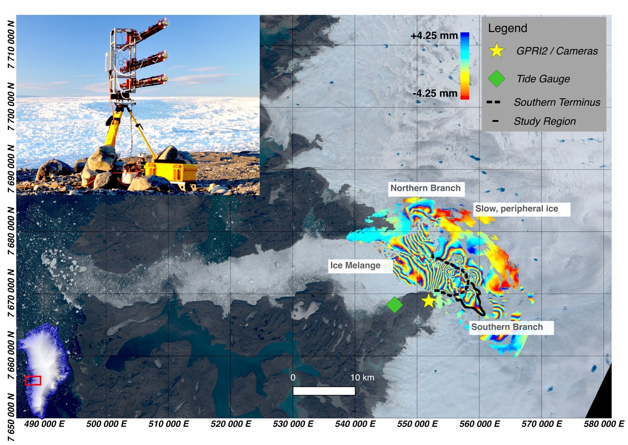
For this project, we used a terrestrial radar interferometer (TRI) to measure the dynamic response to iceberg calving along Jakobshavn Isbræ. The TRI is capable of measuring millimeter scale surface deformation with ~50 m spatial resolution at distances up to 16 km. It records these observations every few minutes, which makes it an ideal instrument for monitoring tidewater glacier response to short term perturbations, such as iceberg calving, ocean tides, and subglacial discharge. By comparison, modern satellite technology can make similar observations but only about once acquisition every 1 to 2 weeks.
Fast flowing tidewater glaciers
Tidewater glaciers are fast flowing outlet glaciers at the ice-ocean boundary. Ice lost at this boundary accounts for at least half of all ice mass discharged into the ocean from Greenland and nearly all of Antarctica’s ice mass loss. Their calving fronts (vertical walls from which ice fractures off) are perturbed by several different geophysical processes including: iceberg calving, fjord circulation, ocean tides, and subglacial discharge.
Iceberg Calving
Gaining a better understanding of the iceberg calving process and how it affects glacier flow is critical to understanding the ice mass lost from the major ice sheets and the resultant increase in sea level. One objective of this project was to characterize the dynamic response of this glacier to iceberg calving.
Step Change in velocity due to iceberg calving
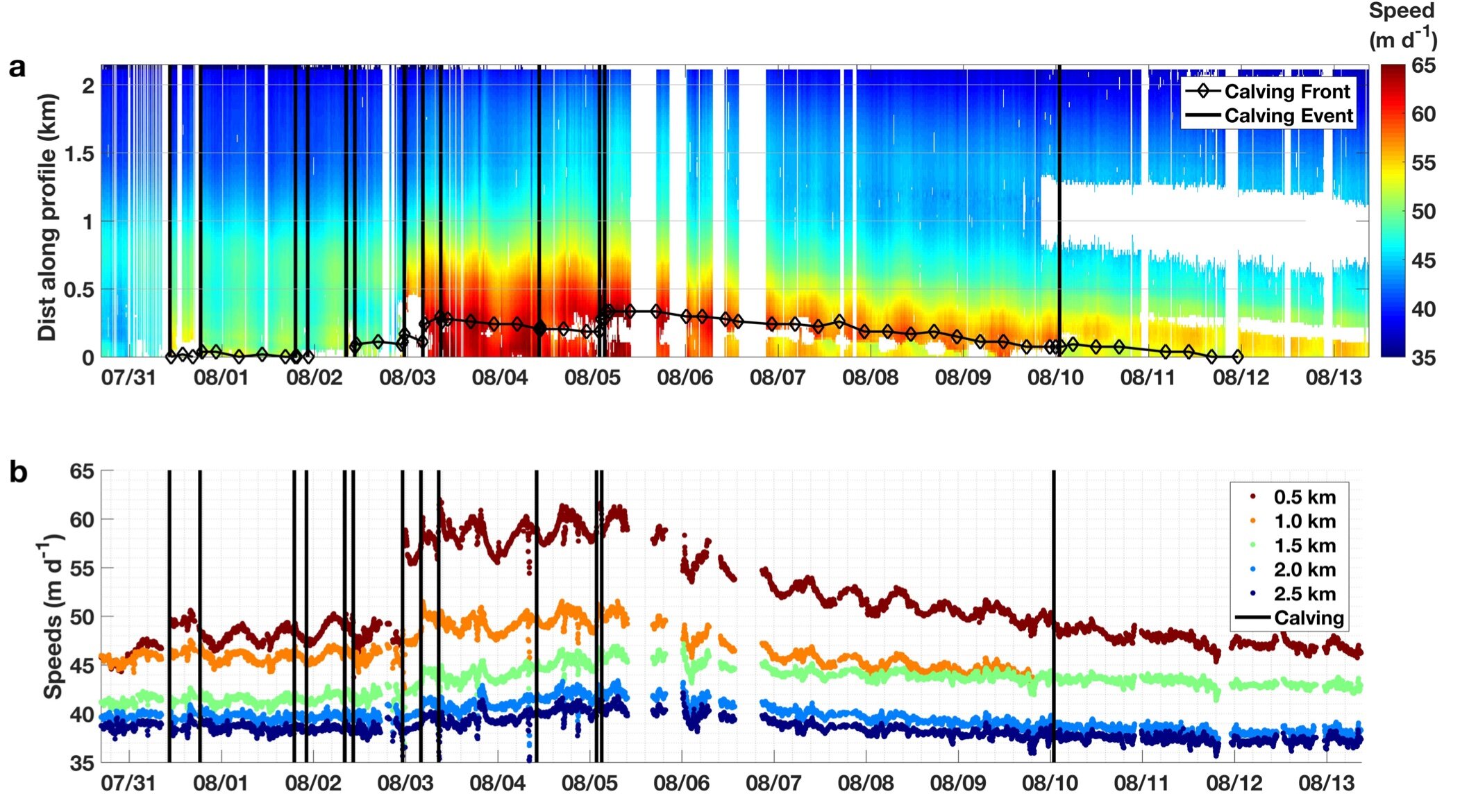
We used the high resolution (~50 m) and fast sampling time (3 mins.) of a terrestrial radar interferometer to characterize the glacier response to iceberg calving. Glacier velocities increased after several calving events, including a step increase in speed late on Aug 2, 2012. The change in speed resulted in some of fastest ice flow ever recorded along a tidewater glacier.

Does calving size matter?
Jakobshavn Isbræ produces some of the largest icebergs in all of Greenland. Indeed, icebergs grounded at the mouth of the fjord (see picture at top of the page) measure kilometers in scale. Interestingly, we found that the largest increase in glacier flow occurred after a relatively small calving event while other larger events had minimal effect on glacier speed. This is contrary to what was expected.
Dynamic response to iceberg calving
Glacier ice is an incompressible material, meaning that once the density of glacier ice reaches ~917 kg/m^3 it cannot be compressed any further. Consequently, glaciers ‘stretch’ as they speed up in a process known as dynamic thinning. In the days leading up to the Aug 2 calving event, a small increase in glacier speed dynamically thinned the glacier nearest the calving front. This helped to sustain moderate speeds, but a compressive stress along the terminus (green patch in row b) likely due to ice held up along a narrow opening in the glacier bed, opposed flow and prevented the glacier from flowing faster. The Aug 2 calving event removed this impeding ice, and the glacier sped up and continued to dynamically thin (row c). As a result, more of the terminus was closer to flotation (row d), which lowered basal resistance to sustain fast flow. Eventually thicker ice further upglacier advected towards the calving front, which increased ice thickness along the terminus, increased basal resistance and caused glacier speeds to slow.

Spatiotemporal variations around 2 August 23:10 calving event. (a) Speeds, (b) longitudinal strain rates (purple = extension, green = compression), (c) surface elevation changes, (d) height above flotation (HAF) with the corresponding (white lines) and 30 July 16:22 (white dashed line) front positions shown for reference.